
Matrix, quaternion and scene graph: Part1
Hi everyone, today I want to speak about math, simply if possible, because the topic is about matrix & quaternion.
The main goal of this series of posts is to use them correctly inside an applied case: the scene graph and how to compute modelview-projection.
Preface
Don’t hesitate to bring more references in the comments.
Source code
I use glm library to manipulate matrix and quaternion. It’s free, it’s only headers (no lib or dll) and it’s cross-platform.
Finally, I use macros EXPECT_EQ and others from Google Test.
All following examples are inside my GitHub https://github.com/Rominitch/myBlogSource/, see Matrix_Quaternion.
Notation
In the following examples, I will use the following writing convention:
- Left to right multiplication
- Row-major order for matrix
Simple notation

Extend notation
![\begin{align*} & {\color{myR}\begin{bmatrix} m_{0} & m_{1} & m_{2} & m_{3} \\ m_{4} & m_{5} & m_{6} & m_{7} \\ m_{8} & m_{9} & m_{10} & m_{11} \\ m_{12} & m_{13} & m_{14} & m_{15} \end{bmatrix}} \\ {\color{myG} \begin{bmatrix} v_{0} & v_{1} & v_{2} & v_{3} \end{bmatrix}} & \mspace{5mu} \bigl[ {\color{myB}\begin{matrix} \makebox[\widthof{$m_{12}$}]{$r_{0}$} & \makebox[\widthof{$m_{13}$}]{$r_{1}$} & \makebox[\widthof{$m_{14}$}]{$r_{2}$} & \makebox[\widthof{$m_{15}$}]{$r_{3}$} \end{matrix}} \mspace{5mu} \bigr] \end{align*}](http://mouca.fr/wordpress/wp-content/ql-cache/quicklatex.com-2fa05004f84263fecda803686527fd67_l3.png "Rendered by QuickLaTeX.com")
Equivalent source code
glm::mat4 matrix(0.0f, 1.0f, 0.0f, 0.0f,
                 1.0f, 0.0f, 0.0f, 0.0f,
                 0.0f, 0.0f, 1.0f, 0.0f,
                 0.0f, 0.0f, 0.0f, 1.0f);
glm::vec4 vector(2.0f, 3.0f, 4.0f, 1.0f);
glm::vec4 result = matrix * vector;So we can write: 

glm::mat4 m(0.5f, 0.0f, 0.0f, 0.0f,
            0.0f, 0.5f, 0.0f, 0.0f,
            0.0f, 0.0f, 0.5f, 0.0f,
            0.0f, 0.0f, 0.0f, 1.0f);
glm::mat4 v(0.0f, 1.0f, 0.0f, 0.0f,
            1.0f, 0.0f, 0.0f, 0.0f,
            0.0f, 0.0f, 1.0f, 0.0f,
            0.0f, 0.0f, 0.0f, 1.0f);
glm::mat4 p(1.0f, 0.0f, 0.0f, 0.0f,
            0.0f, 1.0f, 0.0f, 0.0f,
            0.0f, 0.0f, 1.0f, 0.0f,
            1.0f, 2.0f, 3.0f, 1.0f);

glm::mat4 result = p * v * m;
glm::mat4 mvp(0.0f, 0.5f, 0.0f, 0.0f,
              0.5f, 0.0f, 0.0f, 0.0f,
              0.0f, 0.0f, 0.5f, 0.0f,
              1.0f, 2.0f, 3.0f, 1.0f);
EXPECT_EQ(mvp, result);
EXPECT_NE(mvp, m * v * p);
I don’t know if it is a “true” mathematical writing convention but it’s similar to code and c++/glm order.
For simplification reasons and to have more readable diagrams, we work in Z=0 plane.
We stay in 3D in our logic as well as in our formula.
I have an orthonormal system O with its X axis and its Y axis, Z is oriented toward us.
Units depend on the size of x and y vectors.
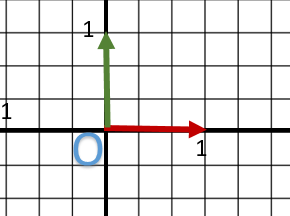
In short, it’s classic.
Transformation matrices
The transformation matrices containing homogeneous coordinates (that we call matrices afterward) allow us to apply a geometric transformation (more or less complexe) to point or vector.
I suppose you either know how to manipulate (basically realize sum/multiplication/transpose/invert) or your software/library can do it for you !
Remind: major forms
Here, you can find the major forms of transformation matrix we want to use:
Translation T
Rotation R
Homothetic or Scaling S


Problem 1: What are transformation matrix ? and how to make them ?
Translation and matrix representation
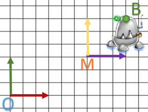
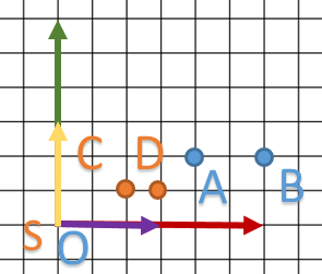
We will start with a rather naive approach. To start with we will try to translate a 3D point.
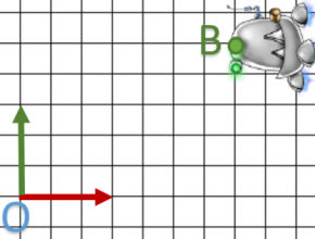
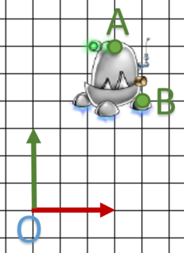
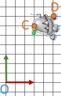
On this diagram, I want to translate my point A to B.
![]()
We can easily read  and
and  so translation vector is
  .
.
We substitute the “t” values of the matrix by this vector and compute the multiplication with A.

glm::vec4 b( 3.0f, 2.0f, 0.0f, 1.0f);

glm::vec4 a( 1.0f, 1.0f, 0.0f, 1.0f);
glm::mat4 t( 1.0f, 0.0f, 0.0f, 0.0f,
             0.0f, 1.0f, 0.0f, 0.0f,
             0.0f, 0.0f, 1.0f, 0.0f,
             2.0f, 1.0f, 0.0f, 1.0f );
EXPECT_EQ( b, t * a );

glm::mat4 t2( 1.0f ); // Identity
t2 = glm::translate( t2, glm::vec3( 2.0f, 1.0f, 0.0f ) );
EXPECT_EQ( b, t2 * a );
Finally, we retrieve our point B but …
- It looks like it worked, but what really happended ?
- Is it really more complex than applying a translation vector ?
- What did we use the other parts of the matrix for ?
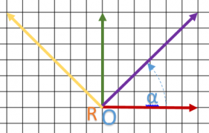
Now things are getting more difficult because we don’t actually apply a translation. It’s more like changing our point of view. We are looking at the same object but from a different place.
Actually, matrices allow to change the coordinate system.
I call  system, a system defined by X origin and
  basis.
The real form is:

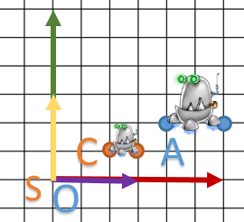
This is the “actual” diagram of what happened:
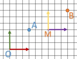
In fact, our translation matrix will create another basis M with x,y,z vectors similar to O basis. We notice that:
 so the initial drawing (here just a point) doesn’t move in relation to basis.
- B coordinates are written in
 basis.
There is sill one last question we need to answer: If B coordinates are written in O basis, in which basis is A written ?
The answer is simple: inside M basis.
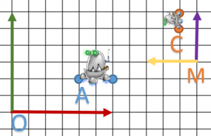
It has its own system
 and a point
  representing the eye.
 .
.and another
 which hierarchically depends from O because point M is defined in O system.), I will transform my point E to A for O system or B for M system.
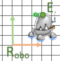
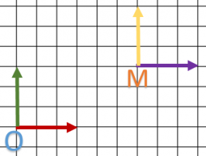
Finally, we defined both O and M system. A point is defined in M system and B in O. Our matrix realized a transformation from M to O system.
is upper system of because M coordinates are defined in : we have a hierarchy notion.
We have just added an important notion: the application way.
In order to change it, we need to invert the matrix. Indeed, all the previous transformation matrices are invertible.
To conclude:
- Matrices represent a change of basis between two systems in the same hierarchy
- Its has a way of application: up or down into hierarchy
For what follows, we will create all our matrix in this way: current to up because they are more intuitive to create.
World is mainly the top of the hierarchy.
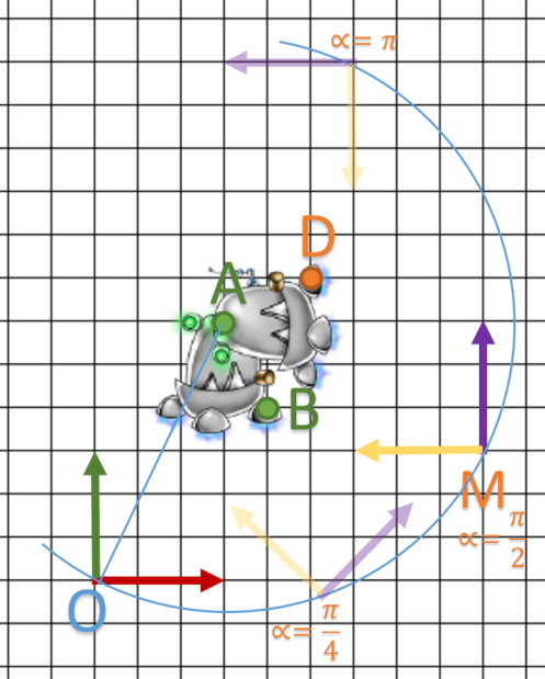
The rotation
The rotation matrix allows us to define the basis of our system. Each vector is normalized before being used inside the matrix.
We have the following matrix:

It’s very simple to write rotation matrix of  around
  .
.
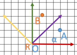
We start with this diagram:
Reading coordinate, we have  ,
,  and
and  .
.
I define  soit
soit  which allows me to normalize vectors.
 . For those who know their rotation matrix around
  , by hearth sin() et cos() are here.
I integrate normalized vectors into the matrix and I have:

const float pi_4 = 0.785398163397448309616f;
const float C = 1.0f / sqrt(2.0f);
// Made hand matrix
glm::mat4 r( C,    C,    0.0f, 0.0f,
            -C,    C,    0.0f, 0.0f,
             0.0f, 0.0f, 1.0f, 0.0f,
             0.0f, 0.0f, 0.0f, 1.0f);

// Or using glm
glm::mat4 r1(1.0f); // Identity
r1 = glm::rotate(r1, pi_4, glm::vec3(0.0f, 0.0f, 1.0f));

EXPECT_EQ(r, r1);
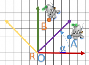
Let’s try to play with this example:  and
and  (it is simple enough to compute using Pythagore theorem only and in noticing than OA = y coordinate of point B)
![\begin{align*} & \begin{bmatrix} {\color{myM} C} & {\color{myM}C} & {\color{myM}0} & 0 \\ {\color{myY}-C} & {\color{myY}C} & {\color{myY}0} & 0 \\ {\color{myB} 0} & {\color{myB}0} & {\color{myB}1} & 0 \\ 0 & 0 & 0 & 1 \end{bmatrix} \\ {\color{myR}\begin{bmatrix}\frac{2}{3} & \frac{1}{3} & 0 & 1\end{bmatrix}} & \mspace{5mu} \bigl[ {\color{myB}\begin{matrix} \makebox[\widthof{$-C$}]{$\frac{C}{3}$} & \makebox[\widthof{$C$}]{$C$} & \makebox[\widthof{$0$}]{0} & \makebox[\widthof{$1$}]{1} \end{matrix}} \mspace{5mu} \bigr] \end{align*}](http://mouca.fr/wordpress/wp-content/ql-cache/quicklatex.com-4b45b3956ba66dced3792ae94e7e9690_l3.png "Rendered by QuickLaTeX.com")
const float C = 1.0f / sqrt(2.0f);
glm::mat4 r( C,   C,    0.0f, 0.0f,
            -C,   C,    0.0f, 0.0f,
            0.0f, 0.0f, 1.0f, 0.0f,
            0.0f, 0.0f, 0.0f, 1.0f);

glm::vec4 a(2.0f/3.0f, 1.0f/3.0f, 0.0f, 1.0f);
glm::vec4 b(   C/3.0f, C,         0.0f, 1.0f);

EXPECT_EQ(b, r * a);
Perfect ! We did it !
Some remarks:
- Rotation turns around the origin of R.
- We can “easily” verify that a matrix is correct (see if X/Y/Z vector is positive/negative on each component).
- B coordinates are system (as expected).
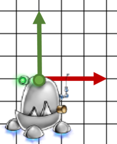
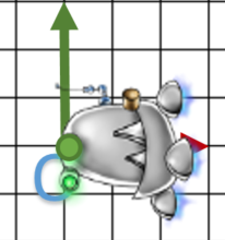
On complex model (many points), rotation will give you:
Another question is raised: how to turn around another point ? Ok … I leave it for now but you have the reply at the end of the post.
and finally homothetic transformation
Here, we want to “stretch” our object into each dimension. For that, we applied on each basis’ vector a scaling factor.
Each scaling factor is defined in  .
.
When superior to 1 : we increase, and between 0 and 1 : we reduce.
In this example, we try to reduce or system by two in all dimensions.
This time we take two points in order to see what happens.
- A will become C
- B will become D

glm::vec3 h(0.5f, 0.5f, 0.5f);
glm::mat4 m(h.x,  0.0f, 0.0f, 0.0f,
            0.0f, h.y,  0.0f, 0.0f,
            0.0f, 0.0f, h.z,  0.0f,
            0.0f, 0.0f, 0.0f, 1.0f);

glm::mat4 m1(1.0f); // Identity
m1 = glm::scale(m1, h);
EXPECT_EQ(m1, m);

glm::vec4 a(2.0f/3.0f, 1.0f/3.0f, 0.0f, 1.0f);
glm::vec4 b(1.0f, 1.0f/3.0f, 0.0f, 1.0f);

glm::vec4 c(1.0f/3.0f, 1.0f/6.0f, 0.0f, 1.0f);
glm::vec4 d(1.0f/2.0f, 1.0f/6.0f, 0.0f, 1.0f);

EXPECT_EQ(c, m * a);
EXPECT_EQ(d, m * b);
To conclude, let’s try it on our robot.
Some remarks:
- C and D coordinates are in system.
- Our robot has not moved according to his coordinate system: C coordinates are always at
 of X vector and D at the end of the vector.
To conclude this first part, we saw than matrix creation is not really complicated despite the fact that rotation demands some computation but analize is accessible (during debug phase).
Problem 2: Composition
Generally, the most important is to quickly apply all these operations to our billion points. So the main idea is to create only one matrix with allthe operations inside.
To create them we use composition which is a multiplication between matrices.
MATRIX PRODUCT IS NOT COMMUTATIVE:
 !
!First we try to compose each matrix which define a complete system (translation / rotation / homothetic).
So, the order of the operations are very important but the rules are simple:

So to simplify this post, I will call them: matrices HRT.
As usual, I will take a example to see what happens.
Ok, first, we compute composition.

const float PI = 3.14159265358979323846f;

glm::mat4 s = glm::scale(glm::mat4(1.0f), glm::vec3(0.5f, 0.5f, 0.5f));
glm::mat4 r = glm::rotate(glm::mat4(1.0f), PI*0.5f, glm::vec3(0.0f, 0.0f, 1.0f));
glm::mat4 t = glm::translate(glm::mat4(1.0f), glm::vec3(11.0f/6.0f, 0.5f, 0.0f));

glm::mat4 m(0.0f,       0.5f, 0.0f, 0.0f,
           -0.5f,       0.0f, 0.0f, 0.0f,
            0.0f,       0.0f, 0.5f, 0.0f,
            11.0f/6.0f, 0.5f, 0.0f, 1.0f);
glm::mat4 c = t * r * s;

// Near expected
for(int rawID=0; rawID < 4; ++rawID)
{
    for(int columnID=0; columnID < 4; ++columnID)
    {
        EXPECT_NEAR(m[rawID][columnID], c[rawID][columnID], 1e-6f);
    }
}
If we use it on  .
.
![\begin{align*} & \color{myM}{\begin{bmatrix} 0 & \frac{1}{2} & 0 & 0 \\ -\frac{1}{2} & 0 & 0 & 0 \\ 0 & 0 & \frac{1}{2} & 0 \\ \frac{11}{6} & \frac{1}{2} & 0 & 1 \end{bmatrix} } \\ {\color{myR}\begin{bmatrix}\frac{2}{3} & \frac{1}{3} & 0 & 1\end{bmatrix}} & \mspace{5mu} \bigl[ {\color{myB}\begin{matrix} \makebox[\widthof{$-\frac{1}{2}$}]{$\frac{5}{3}$} & \makebox[\widthof{$\frac{1}{2}$}]{$\frac{5}{6}$} & \makebox[\widthof{$0$}]{0} & \makebox[\widthof{$1$}]{1} \end{matrix}} \mspace{5mu} \bigr] \end{align*}](http://mouca.fr/wordpress/wp-content/ql-cache/quicklatex.com-5bc271507db4401c3132b0182e7069db_l3.png "Rendered by QuickLaTeX.com")
glm::mat4 m(0.0f,       0.5f, 0.0f, 0.0f,
           -0.5f,       0.0f, 0.0f, 0.0f,
            0.0f,       0.0f, 0.5f, 0.0f,
            11.0f/6.0f, 0.5f, 0.0f, 1.0f);
glm::vec4 a(2.0f/3.0f, 1.0f/3.0f, 0.0f, 1.0f);
glm::vec4 b(5.0f/3.0f, 5.0f/6.0f, 0.0f, 1.0f);

glm::vec4 mul = m * a;

// Near expected
for(int columnID=0; columnID < 4; ++columnID)
{
    EXPECT_NEAR(b[columnID], mul[columnID], 1e-6f);
}
Now, we can “translate” complex system to matrix, but we need to compose many systems based on hierarchy. So we take another example.
Turn around another point
Previously, I told you rotation matrix turn around the origin of a local system. Sometime we need to change it: I will show you the methodology.
 .
.
 .
.
Finally, we realize: one translation + one rotation + one translation.
We see how to make HRT matrix but can we combine more of them?
Let’s try:

Using this example:  and
and  some points of our object, we try to apply a rotation of
  around A.
We expect  and
and 
Start with composition matrix:

const float PI = 3.14159265358979323846f;

glm::mat4 m( 0.0f, 1.0f, 0.0f, 0.0f,
            -1.0f, 0.0f, 0.0f, 0.0f,
             0.0f, 0.0f, 1.0f, 0.0f,
             3.0f, 1.0f, 0.0f, 1.0f );

glm::mat4 op = glm::translate( glm::mat4( 1.0f ), glm::vec3( 1.0f, 2.0f, 0.0f ) );
glm::mat4 po = glm::inverse( op );
glm::mat4 r  = glm::rotate( glm::mat4( 1.0f ), PI*0.5f, glm::vec3( 0.0f, 0.0f, 1.0f ) );

glm::mat4 c = op * r * po;

// Near expected
for( int rawID=0; rawID < 4; ++rawID )
{
    for( int columnID=0; columnID < 4; ++columnID )
    {
        EXPECT_NEAR( m[rawID][columnID], c[rawID][columnID], 1e-6f );
    }
}
Now, try it on points
![\begin{align*} & {\color{myM}\begin{bmatrix} 0 & 1 & 0 & 0 \\ -1 & 0 & 0 & 0 \\ 0 & 0 & 1 & 0 \\ 3 & 1 & 0 & 1 \end{bmatrix}} \\ {\color{myG} \begin{bmatrix} \frac{4}{3} & \frac{4}{3} & 0 & 1 \end{bmatrix}} & \mspace{5mu} {\color{myO} \bigl[\begin{matrix} \makebox[\widthof{$-1$}]{$\frac{5}{3}$} & \makebox[\widthof{$1$}]{$\frac{7}{3}$} & \makebox[\widthof{$0$}]{$0$} & \makebox[\widthof{$0$}]{$1$} \end{matrix} \mspace{5mu} \bigr]} \end{align*}](http://mouca.fr/wordpress/wp-content/ql-cache/quicklatex.com-7a3bc6d58bb560df2973dbb9f2e25b1a_l3.png "Rendered by QuickLaTeX.com")
glm::mat4 m( 0.0f, 1.0f, 0.0f, 0.0f,
            -1.0f, 0.0f, 0.0f, 0.0f,
             0.0f, 0.0f, 1.0f, 0.0f,
             3.0f, 1.0f, 0.0f, 1.0f );

glm::vec4 a( 1.0f, 2.0f, 0.0f, 1.0f );
glm::vec4 b( 4.0f/3.0f, 4.0f/3.0f, 0.0f, 1.0f );
glm::vec4 c( 1.0f, 2.0f, 0.0f, 1.0f );
glm::vec4 d( 5.0f/3.0f, 7.0f/3.0f, 0.0f, 1.0f );

EXPECT_EQ( c, m * a );

glm::vec4 computed = m * b;
// Near expected
for( int columnID=0; columnID < 4; ++columnID )
{
    EXPECT_NEAR( d[columnID], computed[columnID], 1e-6f );
}
I leave you the care of computing C and you see we have a good result.
Our solution is easy to understand and intuitive, moreover it demands only one multiplication.
For your information, one last diagram:
To conclude, Our HRT matrices can be composed and cascaded: this is an important subject which helps us when we try to use them into scene graph.
Conclusion
We saw :
- A definition of matrix with homogeneous coordinates
- their main shapes and how to create them
- The composition
Here we have all information to use them into scene graph.
But, I want to speak about quaternions before: ! Wait for the translation !
If you don’t need them: ! Soon !
Thanks for reading!
Don’t hesitate to shared, post a comment/fix in order to make it a dynamic tools !
References
Wikipedia : Produit matriciel
Wikipedia : Transformation matrix
Wikipedia : Matrice de passage
www.opengl-tutorial.org – Tutorial 3 : Matrices
Les transformations géométriques du plan
University of Edinburgh – Transformations – Taku Komura